Binding energy from Dirac equation as a function of Z

Date: 2016-03-05

Here we shall plot the electron binding energy predicted by the Dirac equation for the hydrogen atom:

\[E_{nj}=mc^2\left\{\left[1+\left(\frac{\alpha Z}{n-(j+1/2)+\sqrt{(j+1/2)^2-(\alpha Z)^2}}\right)^2\right]^{\frac{-1}{2}}-1\right\}\]

import matplotlib as mpl

params = {
    "font.family": "serif",
    "text.usetex": True,
    "font.serif": 'Palatino',
    "figure.figsize": [5.5,4],
}
mpl.rcParams.update(params)

import numpy as np
from matplotlib import pyplot as plt

# Setting a nice plot style
plt.style.use('ggplot')

# Define a function to calculate E(Z) given j and n

def E(Z,j,n):
    
    # Defining some constants 
    
    c = 3*(10**8) # Speed of light
    m = 9.1*(10**(-31)) # Mass of the electron
    alpha = 137**-1 # Fine structure constant 
    
    # Defining our binding energy function, E(Z) 
    # derived from the Dirac equation.
    
    denom = n - (j + .5) + np.sqrt((j + 0.5)**2 - (alpha*Z)**2)
    frac = alpha*Z/denom
    return m*(c**2)*((1+frac**2)**(-0.5) - 1)  

# Now defining a function to plot E(Z)

def binding_energy_plot(j,n):
    
    # Create an even spaced array of numbers in the range 
    # 0 - 137, in steps of 0.1.
    Z = np.arange(0.0, 137.0, 0.1)  
    
    
    # Plot the function
    plt.plot(Z, E(Z,j,n))
    
    # Label the x and y axies
    plt.xlabel("Z")
    plt.ylabel("Binding Energy (Joules)")
    
binding_energy_plot(0.5,1)     
plt.tight_layout()
plt.savefig('dirac_binding_energy.png')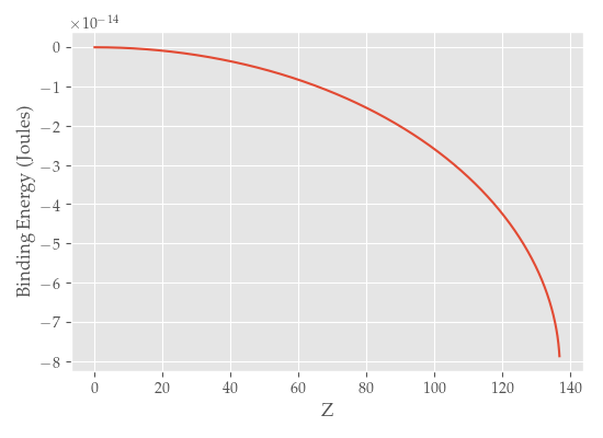

We can see that the binding energy goes asymptotically to \(-\infty\) as \(Z\rightarrow 137\) (that is, as \(\alpha Z\rightarrow 1\)). In this regime, the coupling is so strong that we can have spontaneous production of electron-positron pairs from the vacuum, and we must turn to quantum field theory instead.